Hands-on class on Science & Technology Indicators: Scientific Journals and Journal Structures.
18 April 2007
In a methodological appendix to their study with an evaluation of The Cancer Mission of the US during the 1970s, Studer & Chubin (1980, at p. 269) formulated a crucial question for science and technology studies:
Relationships among journals, individuals, references, and citations can be analyzed in terms of their structural properties. But can one be used as a baseline to calibrate our understanding of another? Does it make sense to attempt to “control” for one relationship while studying others? What would be meant by “controlling for ideas” or “controlling for cocitations?” If disparate dimensions of science are not carefully analyzed in their own terms, the possibility of relating their respective contributions is nil.
The authors call for social network analysis as a tool for the methodological approach, but theoretically their empirical research results do not allow them to draw conclusions because in such a complex dynamics the feedback loops disturb any causal scheme.
Evolutionary theorizing, however, distinguishes between variation and selection. Variation may be pre-structured by selection (Dosi, 1982), but nevertheless one can expect variation to be changing more rapidly than selective structures. Selection is deterministic (determined by the structure of the selecting system), while variation introduces randomness (exploration). The selective structures in science are provided by the networks of ideas which are retained in journal articles and their relations.
Two weeks ago, we have looked at relations among texts provided by words and co-occurrences of words; scientific articles additionally contain citations. Citations serve the codification and the retrieval (Fujigaki, 1998). Aggregated journal-journal relations are made available by the Institute of Scientific Information (ISI) in an additional volume of the Science Citation Indices (SCI, SoSCI, AHI) called the Journal Citation Reports (JCR). (There is no JCR for the Arts & Humanities Citation Index.) The JCRs are brought online at http://portal.isiknowledge.com/portal.cgi?DestApp=JCR&Func=Frame since 1998, but are available on CD-Rom since 1994. (Before that we had microfiche and printed issues which are still available at various libraries.)
One can use aggregated citation structures among journals for mapping the intellectual development of scientific and technological fields at a high level of aggregation (Leydesdorff, 1987 and 2006). However, there is no one single best way for doing so: different thresholds, parameter choices, clustering algorithms, etc., may lead to different results. Yet, during the last decades scientometricians have reached increasingly consensus about some basic premises.
The Journal Citation Reports
Let us turn to the website of the JCRs. It is not so easy to find the journals of science, technology, and innovation studies using the subject categories provided. Try to find some of the journals which you know; for example, under the heading “History and Philosophy of Science.” Research Policy is to be found under “Management” and Scientometrics is part of the Library and Information Science literature. Thus, let’s take the other approach of a specific journal, for example, Research Policy. Type the journal name and a new screen is provided which informs us about standard journal indicators like the impact factor, etc.
Click on the journal name. In the new screen, the ISI provides a wealth of information about the journal. Among other things, the different indicators are defined. Try to understand the impact factor or turn to Wikipedia for more information if you fail to grasp the definition from the formulas (at http://en.wikipedia.org/wiki/Impact_factor ). If you inspect the citations to the journal per year, how many years would you than take as a citation window for assessing the influence of a paper in terms of expected citations? Scientometricians use different citation windows, for example, three years. Would you consider this as a wise choice? Why or why not?
OK, let’s move on. Click on the link for the “Cited journal data.” The cited journal tables and citing journal tables, respectively, provide all the basic information which one needs for constructing a citation matrix among journals included in the ISI databases. For example, you can see that Research Policy is cited in total 74 times by articles in Scientometrics and 30 times by articles in Social Studies of Science. In total, Research Policy is cited 2,470 times during 2005. As you can find by proceeding to the next pages, these citations are provide by a large number of journals (165), but only twenty or thirty of these journals contribute substantively to the citation pattern.
Network analysis
Journal citations occur in dense cluster of journals which cover specialties, but most journals have also long tales of the distribution. Thus, Research Policy is cited by articles in Research-Technology Management only twice, and vice versa this latter journal is cited four times by articles in Research Policy. A citation matrix can be constructed by feeding these numbers into a table or an Excel sheet as follows:
|
Citing Cited |
Research Policy |
Res-Techn. Management |
Scientometrics |
|
Research Policy |
432 |
2 |
35 |
|
Res-Techn. Management |
4 |
34 |
0 |
|
Scientometrics |
74 |
0 |
520 |
The zeros are not real zeros, but missing values. All values lower than two are lumped together under the category “All others”. Can you add Social Studies of Science to this table?
The resulting file can be represented in the DL-format (data definition language) which social network analysts use as follows:
DL
NR=4, NC=4
FORMAT = FULLMATRIX DIAGONAL PRESENT
ROW LABELS:
ResTechnolManage
Scientometrics
SocStudSci
ResPolicy
COLUMN LABELS:
ResTechnolManage
Scientometrics
SocStudSci
ResPolicy
DATA:
34 0 0 4
0 520 21 35
0 25 100 7
2 74 30 432
Table 1: Citation matrix in DL format.
Save this file as an ASCII text file and read this into Pajek. Draw the picture. Set the lines at different width. You will see that Pajek reads an asymmetrical (or 2-Mode) matrix like this one as a double matrix. The positions of the cited and citing journals are different and strongly connected because of the high values on the main diagonal.
One can distinguish cited and citing in Pajek by using Net > Partition > 2-Mode. Now two partitions are created of each four journals. If you draw the partitions now, you should see different colours for cited and citing positions. You can change these colours by going to Options > Colors > Partition Colors. If you go back to main menu, go to Partition > Make Cluster > “1”, redraw the partition and under Options > Mark Vertices Using > Mark Cluster Only, you will be able to visualize the (cited or citing?) patterns exclusively. Which patterns do we obtain: the cited or citing ones?
One can also extract partition 1 in the main menu as follow: Operations > Extract from Network > Partition 1. Why does the resulting picture show no relations?
Go back to the original 2-mode network (nr 1.) with 8 nodes. Choose Net > Transform > 2-Mode to 1-Mode. If you choose now Rows, you get the cited patterns; if you choose Columns the citing ones. How are they different or similar?
From Pajek to SPSS and vice versa
In previous lessons we have used the cosine-matrices instead of the raw scores. We will now go from the citation matrix to the cosine matrix using SPSS. In Table 2, the resulting cosine matrix is provided in the format of Pajek itself. But let’s do the exercise in order to understand the relations.
Return to the two-mode matrix with 8 nodes in Pajek (before the further processing). Click on Tools > SPSS > Current Network. Pajek opens a window which reports to you where you can find the file which you need for importing the data into SPSS. Find that file and double click on it. If it works, SPSS opens several windows. (If not, open SPSS, open the file as a syntax file, and Run > All.) In the matrix (in another window), you should find the same information as above, but now within SPSS. Inspect the matrix both in the variable and the data view. Try to understand it fully. The variable view describes the variables and, among other things, labels them.
SPSS computes almost exclusively in terms of variables, that is, columns of the matrix. (We shall see an exception to the rule below.) Cases (rows) can be selected, grouped, and clustered, but are not the subject of analysis. Social Network analysis (Pajek) tends to “think” in terms of the rows. In the analysis above (using Pajek), for example, the rows were the first partition, and the columns the second. The rows represent the nodes and the columns the links attributed to them. Attributes can be variables and thus SPSS “thinks” the other way around. However, you can tumble the matrix (“transpose” it) in both programs.
Let’s make the cosine-matrix. Click on Analyze > Correlate > Distances. Bring the four variables (col1 to col4) to the right side. Compute distances between variables, using Similarities and Choose the cosine instead of the Pearson correlation. The Proximity matrix which is created, contains the cosine values. You can right-click on it and export it, for example, as an Excel file. I pasted the values of this matrix into Table 2 and added the headings in the so-called Pajek-format. This matrix is symmetrical and thus we need the labels only once. Try to replace my values with yours, take the file and import it into Pajek by saving it first as an ASCII Plain text file (DOS with CR/LF, that is “carriage return and line feed” as with the old type-writers).
*Vertices 4
1 "ResTechnolManage"
2 "Scientometrics"
3 "SocStudSci"
4 "ResPolicy"
*Matrix
1.000 0.008 0.017 0.068
0.008 1.000 0.279 0.221
0.017 0.279 1.000 0.312
0.068 0.221 0.312 1.000
Table 2: Cosine values for the citing patterns of four journals.
One can directly import an Excel file into Pajek using the program CreatePajek available at http://vlado.fmf.uni-lj.si/pub/networks/pajek/howto/excel2Pajek.htm .
Mapping science and technology using journal structures
After importing this file into Pajek, the results are at first a bit disappointing because all the relations have values. (The cosine runs from 0 to 1.) Would we have chosen the Pearson correlation some of the relations would have been negative, but for various reasons scientometricians prefer to use the cosine for the visualization (Ahlgren et al., 2003). (For further statistical analysis, the Pearson may be the better choice.)
Go to the main menu in Pajek and under Net > Tranform > Remove > Lines with values lower than 0.2 . Redraw.
At http://www.leydesdorff.net/jcr05 , the Pajek files are provided for the citation environments of all the journals included in the Science Citation Index and the Social Science Citation Index with this threshold of 0.2. Scroll down to Research Policy, save the file as a text file, and import it into Pajek. The file contains the citation environment of all the journals which cite Research Policy to the extent of more than one percent of its total citations. Remember from above that the total citations of Research Policy were 2,470. One percent is 24.7, and thus the 23 journals citing more than 24 times are included. Cosine values below 0.2 are removed in order to enable the user to generate from these files easily a meaningful picture.
After making partitions using the core-option and removing partition zero (using the techniques explained above), you should be able to obtain a picture like this:
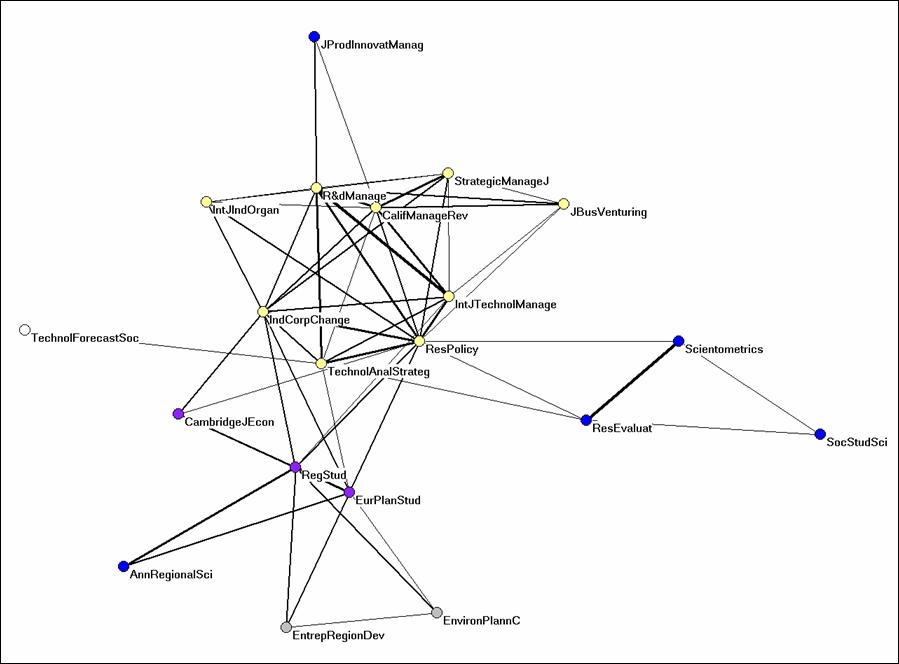
Can you provide this with an interpretation? Note that the relation between Social
Studies of Science and Research Policy is no longer a direct one,
but both of these two journals share a pattern of being cited by authors with
papers in Scientometrics and Research Evaluation.
The data in the file which you downloaded from the webpage contains additional information about the relative share of the citations of the journals. After each label an x-factor and an y-factor are specified. You can turn this additional information on by using Options > Size > of Vertices defined in input file. You may have to adjust the size. The nodes are now depicted proportional to the y-factors and the x-factors in the input file. The y-factor provides the percentage of the citations in this local environment, and the x-factor this same percentage after correction for “within-journal self-citations,” that is, the value on the main diagonal of the citation matrix. What do you see if you turn this on? Export this picture and make it part of the submission for the third mid-term by importing the picture into Word.
Let’s finally do the same exercise for the citing file which you can find at http://www.leydesdorff.net/jcr05/citing . How are the citing patterns different from the cited, and why?
Repeat the analysis for a journal which is central to your own research interests. Can you learn something about the structure of this field?
Reading for next week: http://www.faculty.ucr.edu/~hanneman/nettext/C10_Centrality.html (Hanneman & Riddle, 2005). Don’t pay too much attention to the details. I wish you to understand the difference between degree centrality, closeness, and betweenness centrality.
Loet Leydesdorff
Amsterdam, 18 April 2007
References:
Ahlgren, P., Jarneving, B., & Rousseau, R. (2003). Requirement for a Cocitation Similarity Measure, with Special Reference to Pearson’s Correlation Coefficient. Journal of the American Society for Information Science and Technology, 54(6), 550-560.
Dosi, G. (1982). Technological Paradigms and Technological Trajectories: A Suggested Interpretation of the Determinants and Directions of Technical Change. Research Policy, 11, 147-162.
Fujigaki, Y. (1998). Filling the Gap Between Discussions on Science and Scientists’ Everyday Activities: Applying the Autopoiesis System Theory to Scientific Knowledge. Social Science Information, 37(1), 5-22.
Hanneman, R. A., & Riddle, M. (2005). Introduction to social network methods. Riverside, CA: University of California, Riverside; at http://faculty.ucr.edu/~hanneman/.
Leydesdorff, L. (1987). Various methods for the Mapping of Science. Scientometrics 11, 291-320.
Leydesdorff, L. (2006). Can Scientific Journals be Classified in Terms of Aggregated Journal-Journal Citation Relations using the Journal Citation Reports? Journal of the American Society for Information Science & Technology, 57(5), 601-613.
Studer, K. E., & Chubin, D. E. (1980). The Cancer Mission. Social Contexts of Biomedical Research. Beverly Hills, etc.: Sage.